

Global Gridded Model of Carbon Footprints (GGMCF)
This model provides a globally consistent, spatially resolved (250m), estimate of
carbon footprints (also called Scope 3 emissions) in per capita and absolute terms across 189 countries.
It incorporates existing subnational models for the US, China, Japan, EU, and UK. The model
is described in the open-access publication
Carbon footprints of 13,000 cities.
This article from Scientific American also gives a nice overview of the study. The results have also been covered by
Forbes,
World Economic Forum, NASA's Earth Observatory blog, US News & World Report, National Geographic, among others. The dataset is also available on the WRI ResourceWatch platform (blog).
Key Findings
One observation that can be made based on this model is in many countries, a small number of large and or affluent cities drive a significant share of national total emissions. This means concerted action by a small number of local mayors and governments has the potential to significantly reduce national total carbon footprints. Some other observations based on the results include:
- Globally, carbon footprints are highly concentrated into a small number of dense, high-income cities and affluent suburbs
- 100 cities drive 18% of global emissions
- In most countries (98 of 187 assessed), the top three urban areas drive more than one-quarter of national emissions
- We define cities as population clusters, but in practice mapping footprints to local jurisdictional bounds is complex
- 41 of the top 200 cities are in countries where total and per capita emissions are low e.g. Dhaka, Cairo, Lima). In these cities population and affluence combine to drive footprints at a similar scale as the highest income cities
- For large and high-income cities, their total Scope 3 footprint is much larger than the city's direct emissions
- Radical decarbonization measures (limiting nonelectric vehicles; requiring 100% renewable electricity) can induce substantial emissions reductions beyond city boundaries. In wealthy, high-consumption, high-footprint localities such measures may require only a small investment relative to median income, yet accomplish large reductions in total footprint emissions
- Local action at the city and state level can meaningfully affect national and global emissions
Carbon Footprints of World Cities
The model estimates the carbon footprint (CF) of individual cities. When interpreting the results please keep in mind that the results from a global top-down model will never be as precise as more detailed local or bottom-up assessments. Additionally, defining the city population and bounds is hard. We use the GHS-SMOD definition of "cities" as contiguous population clusters. This does not correspond directly to the precise legal jurisdiction for many cities. Additionally, the population within these clusters may include exurbs and other areas and may not correspond to the city's official population. Taking the city's estimated population as given, model provides results for each city with an associated uncertainty range. The 1 standard deviation value is shown. The mean per-capita CFs are also shown as a median estimate with an associated uncertainty range.
The CF of each cluster is reported as a mean estimate with a standard deviation. These can be interpreted in the normal way: e.g. if the Footprint of a city is reported as 20 ±5, it means there is a 67% chance the city's CF is between 15-25, and a 95% chance the CF is between 10 and 20. Details about how these are calculated are provided in the paper and the SI.
Important note about the city names: The GGMCF is fundamentally based on the EU's GHS-SMOD gridded population model. The urban clusters are identified on top of that gridded population model, and then we attempted to label the cities corresponding to each cluster. To get the city names we use the NORPIL list of cities and ESRI's World Cities database. This matching is not perfectly accurate. In some cases the name is picked up from a closely adjacent city, or from an annex suburb that is contiguous with a larger city. Many clusters we have not yet been able to name; these appear as simply "Unnamed city" in the list.
Below are tables with the top 500 cities, by absolute CF and by CF per capita. See below for download links.
Global results
The global results can be viewed using this interactive map. The lefthand map shows the gridded global carbon footprint, as absolute volume of emissions per grid cell. The top 100 cities are shown (global top 100 in blue, top 50 in orange, and top 10 in red). Open map in new window »
Note: the Web Mercator projection used for this online presentation distorts high-latitude regions (e.g. northern US and European cities), making them appear larger and visually more prominent than they are. All numerical analyses should be done using an equal-area projection. This map was generated with the NTNU Spatial Footprinting Toolbox.
Download results
The top 500 cities in absolute and per capita terms can be donwloaded here as tab-delimited text files:
The complete model can be downloaded as a GeoTIFF file:
- GGMCF_v1.0.tif - absolute emissions per grid cell (200MB compressed, 5GB uncompressed)
- GGMCFPerCap_v1.0.tif - emissions per capita per grid cell (200MB compressed, 5GB uncompressed)

These results are licensed under a Creative Commons Attribution-NonCommercial 4.0 International License.
Please contact us if you would like to use these results for commercial work or if you have an idea for collaboration based on this model.
To cite this work please refer to this paper:
Moran, D., Kanemoto K; Jiborn, M., Wood, R., Többen, J., and Seto, K.C. (2018) Carbon footprints of 13,000 cities. Environmental Research Letters DOI: 10.1088/1748-9326/aac72a.
Technical Summary
The model was constructed using
- the Eora global supply chain database. This was used to determine the national average carbon footprints for 189 countries
- national statistics on urban vs rural household spending patterns (data sources: US BEA, EUROSTAT, World Bank)
- a global map of per-capita purchasing power for 20,159 regions based on local tax statistics collected by MB International
- the GHS-POP 250m gridded population model
- the GHS-SMOD model identifying cities ("high-density population clusters") and towns ("lower density population clusters") worldwide
- existing subnational carbon footprint models for
- USA - details 31,531 ZIP codes - Jones & Kammen (we recommend the CoolClimate Network for city-level results within the USA)
- EU - details 178 mixed NUTS level 1/2/3 regions covering 20 EU countries (Austria, Belgium, Bulgaria, Cyprus, Czech, Denmark, Finland, France, Germany, Greece, Hungary, Italy, Latvia, Malta, Poland, Romania, Slovakia, Slovenia, Spain, Norther Ireland) - Ivanova et al.
- UK - details 408 Local Administrative Districts covering England, Scotland, and Wales - Minx et al.
- China - details 30 provinces - Wang et al.
- Japan - details 47 prefectures - Hasegawa et al.
- India - Work in progress. Resolution - 35 states. Data from Sohail Ahmad, Mercator Institute, based on Ahmad et al.
- Other countries? Please contact us if you have an idea for an additional data source
The above were combined to distribute the carbon footprint of each nation into a spatially detailed gridded model.
Key points of uncertainty are the relative carbon intensity of equivalent expenditure in urban vs. rural areas, the allocation of direct emissions from households, and the typical allocation and aggregation uncertainties associated with the carbon footprints. In the paper we provide results with reliability estimates based on Monte Carlo sensitivity analysis, perturbing the subnational spatial allocation while preserving the national totals.
Defining “cities” is not trivial. In some countries there are up to seven levels of administrative divisions. In the paper we followed the Global Human Settlement Layer, GHS-SMOD. This identifies towns and small urban areas ("low density clusters") as clusters with >5,000 persons and cities ("high density clusters") as contiguously populated areas with >50,000 inhabitants.
The results provide a general view of hotspots and patterns, but to compare the CFs of individual cities or to track how a city’s footprint evolves over time, more detailed accounts based on local data and standardized measures are needed. All individual city footprints presented here should be interpreted with the 1 standard deviation value, which in most cases is substantial (10-100% of the CF itself).
Figures and images

Artistic image showing the total carbon footprint in the Eastern US and Canada. [tweetable JPG] [powerpoint-friendly JPG]
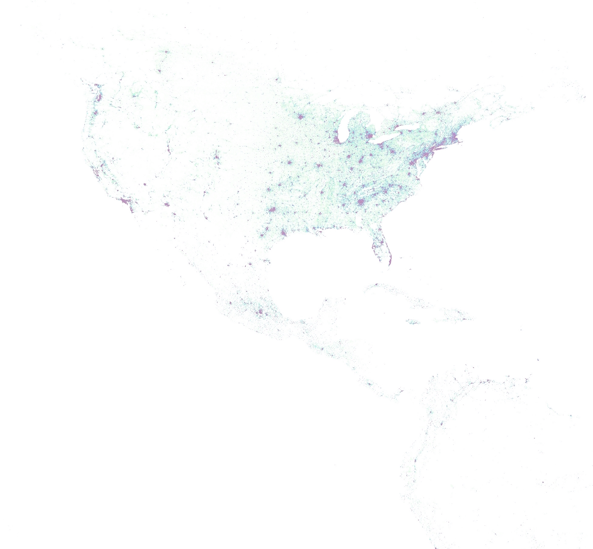
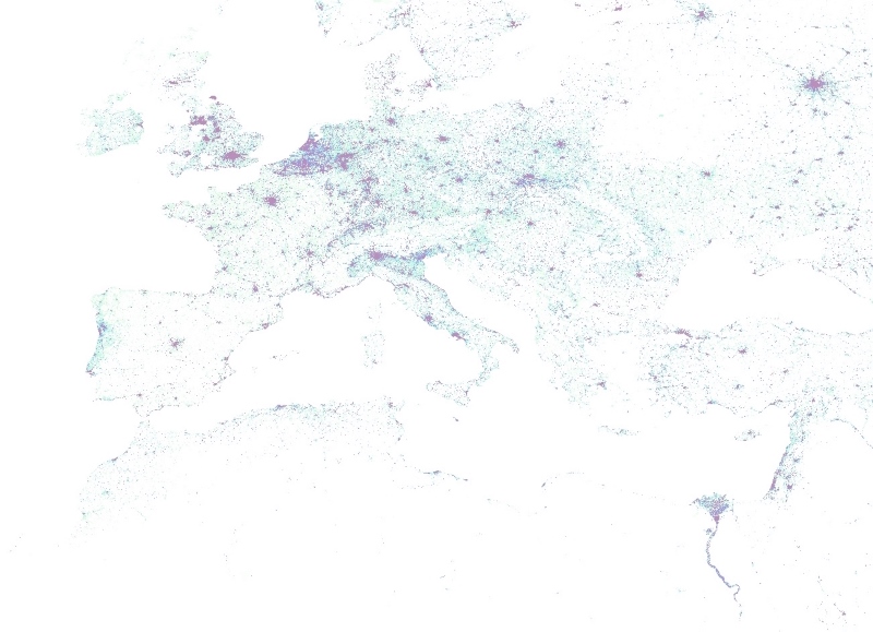
Artistic image showing the total carbon footprint in Europe. [tweetable JPG ] [powerpoint-friendly JPG]
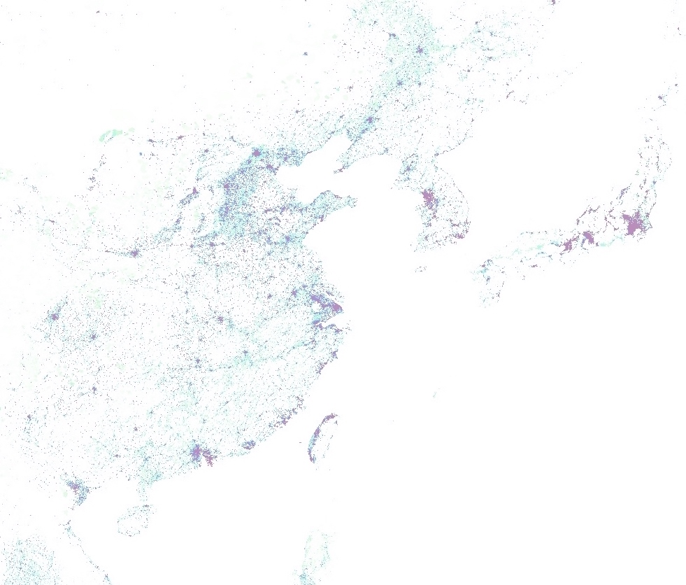
Artistic image showing the total carbon footprint in Southeast Asia. [tweetable JPG] [powerpoint-friendly JPG]
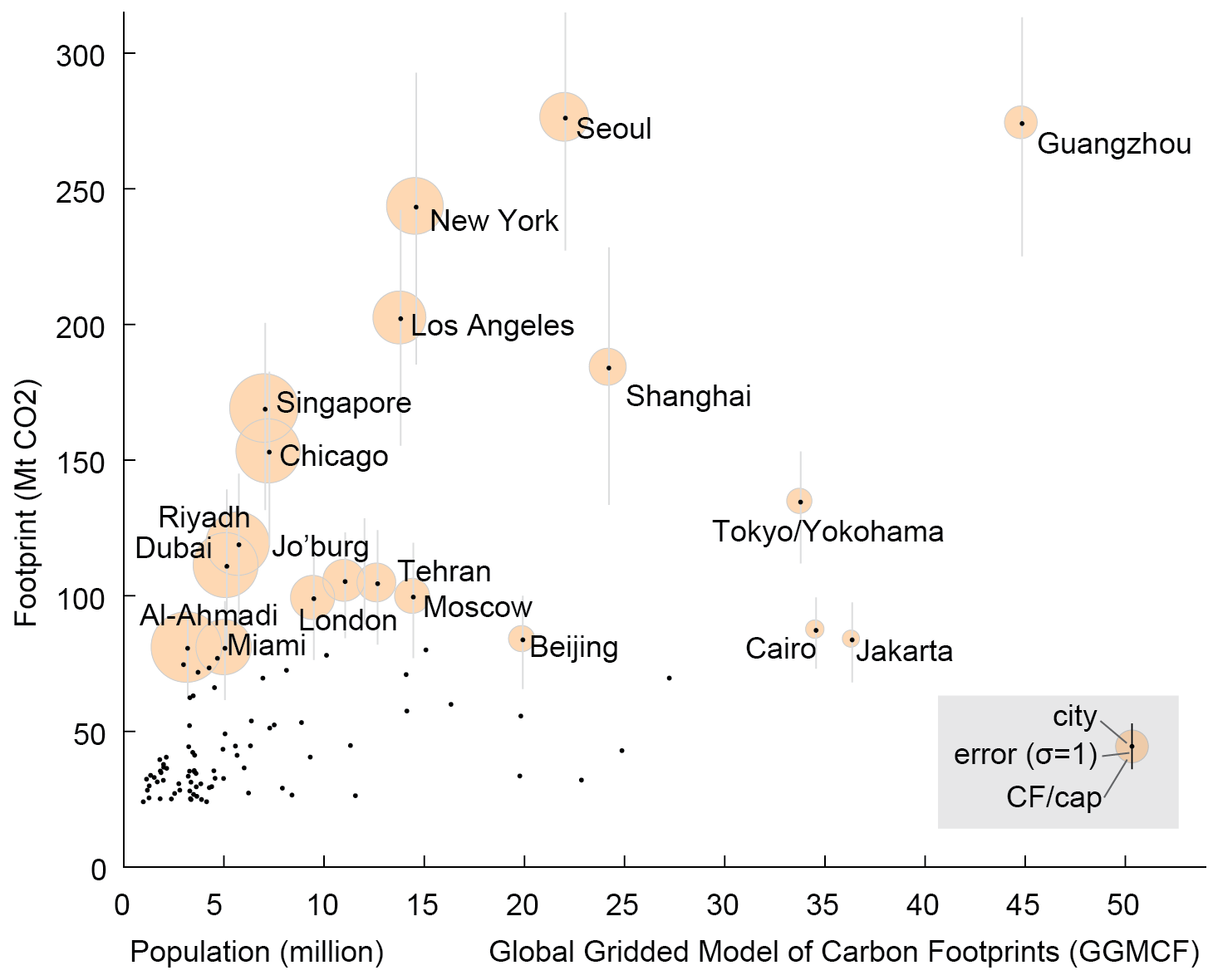
The cities with the largest total footprints (named here are the top 20) have a large CF due to a combination of population and high CF/capita (bubble size). Cairo and Jakarta have relatively low CFs per capita but large populations, while Miami and Al-Ahmadi in Kuwait have smaller populations with higher average footprints, and thus similar total CFs. Vertical lines show 1 standard deviation for each city CF estimate. [PNG SVG
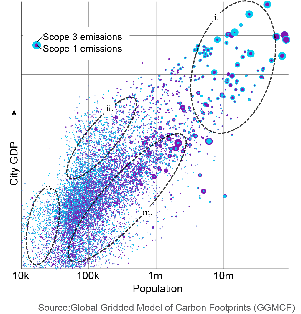
Scope 1 (purple) vs. Scope 3 (blue) emissions, by city Different types of cities: i. populous, high GDP with large footprints (Scope 3>Scope1) include London, Paris, Seoul; ii. smaller, mid-GDP carbon importers, e.g. Oslo; iii. larger, low GDP producers; includes many manufacuturing-intensive Chinese cities; iv. smaller cities, primarily residential, where predominantly Scope 3 > Scope 1. PNG
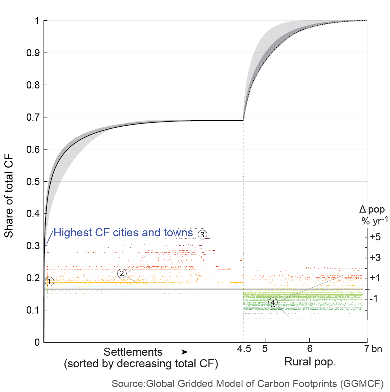
Cities contain 60% of global population and drive 64% of global carbon footprint (CF), but within this the CF is highly concentrated in a small number of high CF cities and high CF/capita suburbs, while populous low CF cities and rural low CF areas contribute relatively little to the total global CF. The lower area shows UN projected growth rates 2020-2050 for each grid cell. The highest growth is expected in low CF cities and declining growth in rural areas, with ① modestly high growth rates around 1-2%/yr for top-CF cities, ② bands visible for cities in India (1.9%) and China (0.6%) across all city sizes, ③ fastest-growing cities currently contributing little to global CF, and ④ declining rural populations all CF/capita, with rural depopulation in Japan (-2.8% capita/yr) visible, but some growth in lower CF/capita regions. PNG SVG
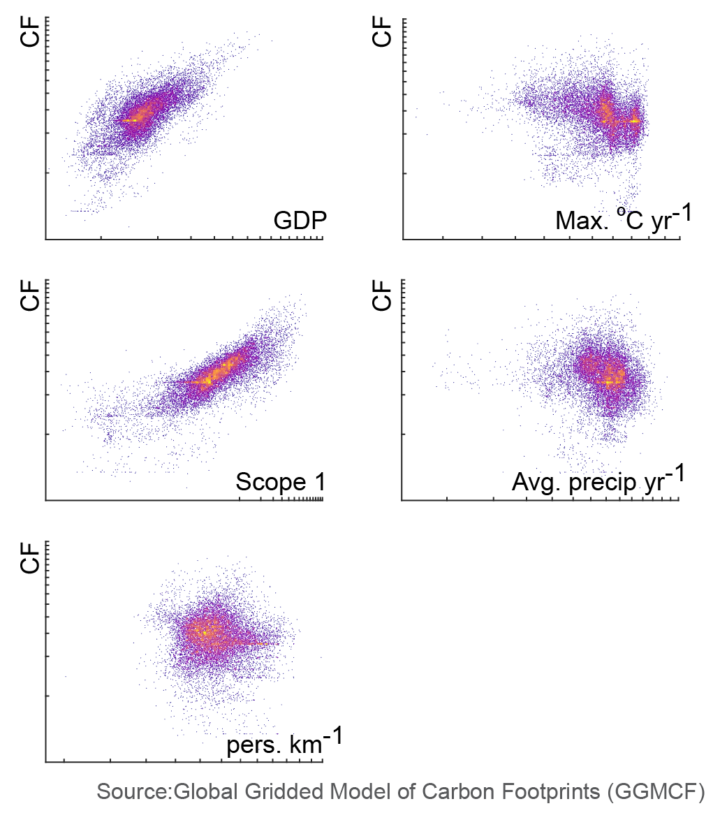
City total Scope 3 emissions are weakly correlated with climate - temperature and precipitation - and population density, but do correlated with GDP and Scope 1 emissions. PNG
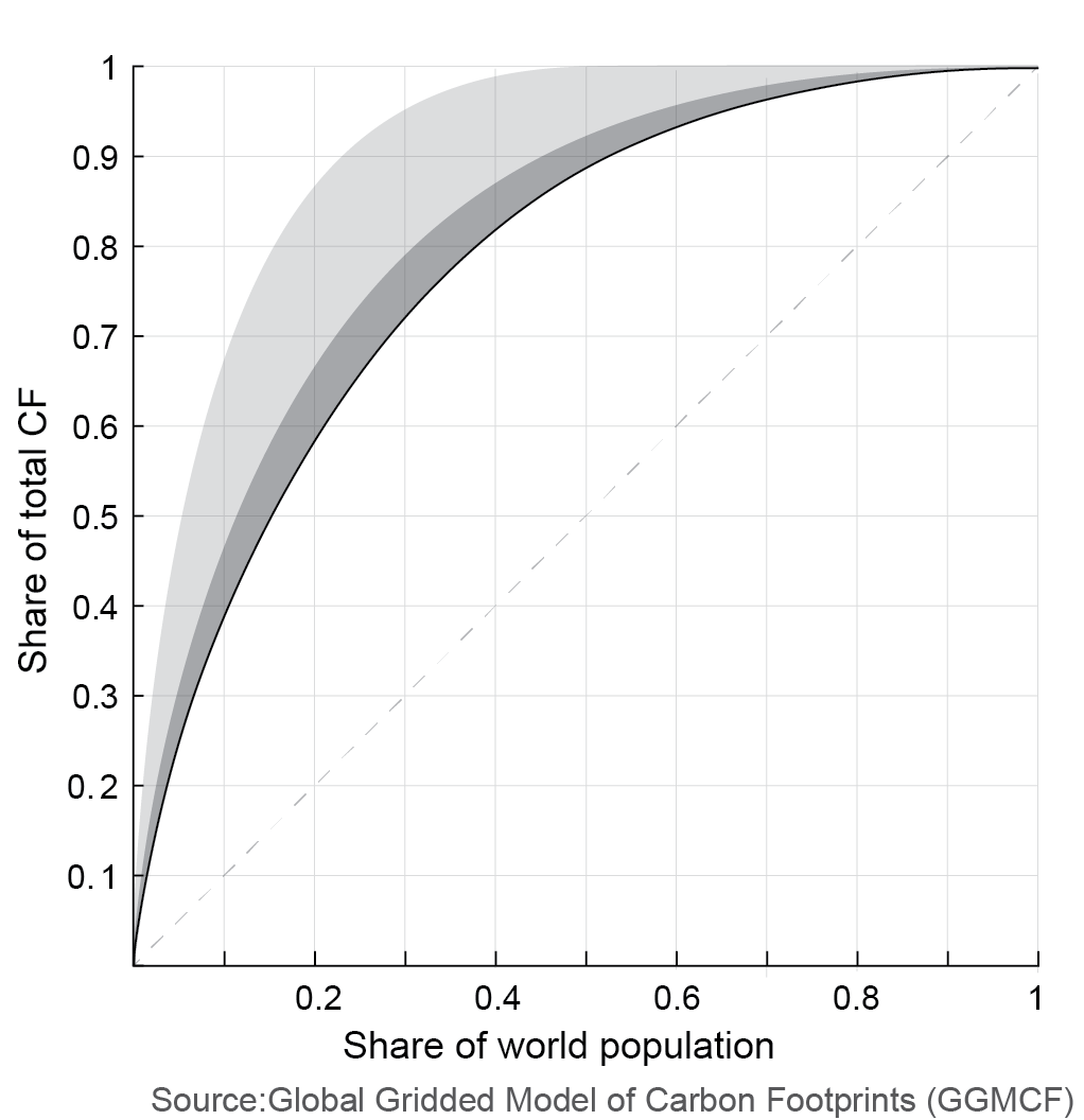
Lorenz curve of gridded carbon footprints shows highest CF/cap decile drives ~40% of global CF CF. The shaded area indicate the range of alternative Lorenz curves constructed during the sensitivity analysis: dark shading indicates individual grid cells were allowed to vary ± 100% and lighter indicates they were allowed to vary ±1000%. (See paper and SI for details.) PNG SVG
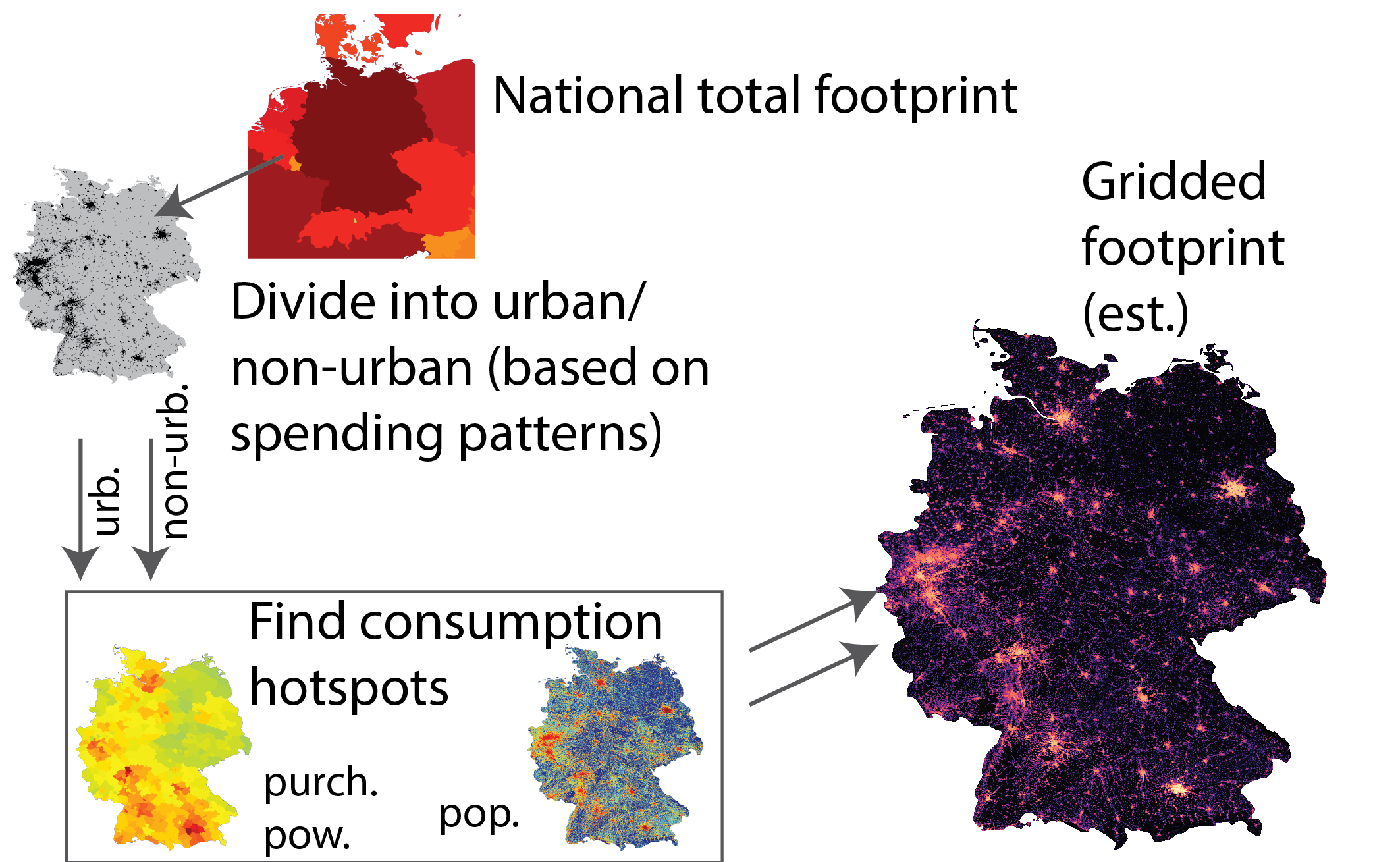
Construction method for gridded model of carbon footprints. The national total footprint (or state/subnational unit footprint for the countries for which subnational data exist) is split in to urban and non-urban components based on relative spending patterns, then spatialized using purchasing power and population. This approach is comprehensive and consistent globally but cannot substitute or individual city footprint accounts based on local data. PNG
Development Team
PI: Daniel Moran - NILU
Collaborators:
Keiichiro Kanemoto - Shinshu University
Magnus Jiborn - Lund University
Richard Wood - NTNU
Johannes Többen - NTNU
Karen C. Seto- Yale
Contributors of subnational models:
Ryoji Hasegawa - Fukuyama City University
Diana Ivanova - NTNU
Chris Jones - UC Berkeley / CoolClimate Network
Jan Minx - Mercator Institute on Climate Change / University of Leeds
Sohail Ahmed - Mercator Institute on Global Commons
Yafei Wang - Beijing Normal University